This was originally posted at The Cameron Hoppe Project.  It’s popularity inspired this site.  It’s been updated since.

          “And He will raise you up on eagle’s wings,

           bear you on the breath of dawn,

           make you to shine like the sun,

           and hold you in the palm of His hand.”

                        — Josh Grobman “On Eagle’s Wings”

At 128+ thousand feet, Baumgartner looks down on the blue sky.

Felix Baumgartner completed his much pre-hyped jump from 128,100 feet, achieving a top speed 1.24 times the speed of sound.  It must have been an amazing ride, with the bill footed by Red Bull and everything.  I am neon green with envy.  Sure, it could be death to try, but it would be worth it just to see the blue-glowing world one time.  Besides, the life insurance is paid.

Gravity creates constant downward acceleration.  Friction with air produces drag that runs the opposite direction in which one is moving, and is proportional to velocity squared.  So the sum of all the forces on Felix, as with any skydiver, during his fall were equal to his mass times his actual acceleration.  Since drag is proportional to the square of velocity, the drag force and the gravitational pull become equal, and acceleration reaches zero.  This is known as terminal velocity.  Not nearly as exciting as the name sounds.  I know; I was disappointed, too.  In equation form it looks like this:

This is a pretty standard force balance on an object moving through a liquid or a gas.

The drag coefficient includes half the surface area of the guy in the suit and a proportionality constant.  Based on his reported time in free fall and an area of 4.3354 square meters I found this to be 1.15, which is actually quite reasonable.

The next issue to deal with in the problem is the air density.  Anybody who’s ever been up a tall mountain or a plane ride knows air gets thinner with elevation.  As a result, drag forces are higher near the ground than at the elevation Baumgartner jumped from. Without that included, we’re only left with the beautiful sky, without any interesting math.  So we can expect that Felix’s speed went way up, and then it actually decreased until he pulled his parachute at 270 seconds.  Then it really dropped.  The air density equation is described below:

Air density is a function of initial pressure, temperature, and height off the ground.

There’s a ton more I just didn’t have time to do.  For example the gravitational force also decreases as elevation increases and the temperature gradient is probably not a constant from the ground to the stratosphere, etc, etc.  But time is short.  Well, we’ve got two coupled differential equations.  There’s only one thing to do–code it and find out how it looks!  I punched this one out in Matlab:

Baumgartner’s position with time into the jump. The green circle marks the point at which his descent slows and the red line is the time where the chute was deployed.

The scale of this is in tens of thousands of feet, so you can see where he pulls the cord at 270 seconds and about 8400 feet.  At that point, his descent slows way down.  Now, the velocity of the fall:

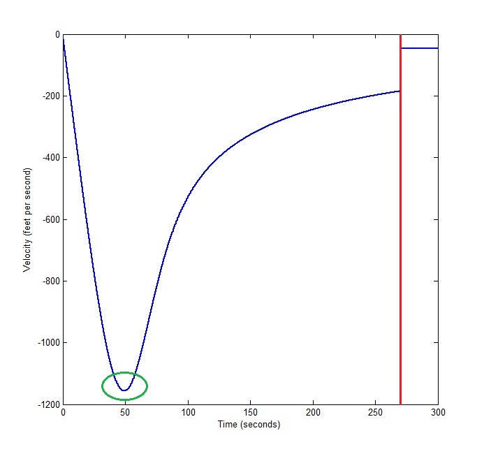
Baumgartner’s Velocity over the time period of the jump. Maximum velocity predicted by the model is too low by about 4.1%.

Two important spots here.  On the right, you can see where his chute deploys.  On the left, you can see where he reached terminal velocity in the upper atmosphere about 50 seconds in.  This was his maximum velocity.  After that, the rising density of the atmosphere continually slowed him down.  Kinda like being married.

You can see the model is a little off; the maximum velocity should be 1223.75 feet per second, while I’ve got him maxing out around 1175.  It’s probably due to my crude modeling of gravitational and temperature gradients at high elevation.  What can I say?  There’s only so many hours in a Sunday afternoon. The model is named for Baumgartner but it can be used generically for any object falling through a gas.  It works out everything in SI units, then converts to feet at the end before plotting.  Changing the plot command to small letters puts it in  SI.  The rest is pretty straightforward.  The function call is:

Baumgart(r,L,CD,p0,u0,a0,rhoR,rho0,T0,Tf)

r = Radius of object         L = Length of object        CD = Drag Coefficient

p0 = initial position       u0 = initial velocity         a0 = initial acceleration

rhoR = density of object        rho0 = density of air at sea level

T0 = Temperature at sea level in Celsius         Tf = Temperature at p0

The call I used was:

Baumgart(0.65,1.9,1.15,39045,0,0,1062,1.48,-25,25)

Cheers!

PS–Are you following @CameronHoppe on Twitter yet?  If you follow me, I’ll follow you.  Plus you should leave a comment.  Just sayin’.

Code:

function Baumgart(r,L,CD,p0,u0,a0,rhoR,rho0,T0,Tf)
tstep = 0.00001;
 Tgrad = (Tf - T0)/30000000;
for n=1:30000001
 t(n) = (n-1)*tstep;
 u(n) = 0;
 p(n) = 0;
 end
n = 0;
for n=1:27000001
 a(n) = 0;
 rho(n) = 0;
 T(n) = 273.15 + T0 + (n-1)*(Tgrad);
 end
a(1) = a0;
 u(1) = u0;
 p(1) = p0;
 rho(1) = rho0*exp(-0.0284877*9.8*p0/(T(1)*8.3144621));
n = 0;
V = pi*L*r^2;
 A = 2*pi*r*(r+L);
 g = -9.8;
 k = 0.5*CD*A;
massR = rhoR*V;
for n=2:27000001
 u(n) = u(n-1) + tstep*a(n-1);
 p(n) = p(n-1) + tstep*u(n);
 rho(n) = rho0*exp(-0.0284877*9.8*p(n)/(T(n)*8.3144621));
 a(n) = (massR^-1)*(V*(rhoR-rho(n))*g + k*rho(n)*(u(n)^2));
 end
uS = u(27000001)*.25;
for n = 27000002:30000001
 u(n) = uS;
 p(n) = p(n-1) + tstep*u(n);
 end
for n = 1:30000001
 P(n) = p(n)*3.28084;
 U(n) = u(n)*3.28084;
 end
 A
 k
 m = plot(t,P);
 xlabel('Time (seconds)')
 ylabel('Position (feet)')
 set(m,'LineWidth',2)